Lessons Learned from Bloomberg's GPT Model Journey

Generative models especially GPT style models have been the front and centre of the conversation for the past few months. There are many factors that contribute to the performance and usability of these models. Perhaps the most important factor is the training data, its quality, distribution and processing pipeline. This has encouraged many institutions to invest in training their internal large language models (LLMs) from scratch or finetune existing open source ones which is still a very expensive operation.
Bloomberg is one of these institutions. The existing LLMs have been trained on massive amounts of data from the internet (and some private data in some cases like ChatGPT) which includes various topics but at the end of the day are too broad to be useful for any specialised domain, e.g. medicine or finance. In addition to the data distribution, the tokenisation step affects how the model learns to interpret the input text. General text LLMs do not use the tokenisers that works best for numbers and therefore the model does not perform well on math and finance-related topics.
These were the main reasons why Bloomberg took up the challenge to train its own GPT LLM. Training such models is no easy feat, you may encounter training instability, scaling issues, deployment and inference challenges, compute, time and budget restrictions. Even if all goes well, which it won't, there is no straight path to determining the right combination of data and parameters and model size. We usually hear about the final polished model and not so much about the many iterations and decisions made that lead to it.
Bloomberg has published an extensive paper on these very topics which I will go over some in this blog post.
Dataset
A combination of general language public data and in-house private finance data is used.
Proprietary finance data - FinPile
Finpile as Bloomberg calls it, is a set of financial documents accumulated over the years from 2007 - 2022 and makes up 51.27% of the entire training dataset or 363B tokens.
Public data
Three public datasets are included in different proportions. For example, C4 (Colossal Clean Crawled Corpus) makes up 19.48% or 138B tokens. Other public datasets used are The Pile and Wikipedia. Total number of tokens from these sources are 345B.
Tokenisation
Handling numbers is a necessity for a language model with financial use cases. It needs to have a good understanding of comparisons, basic arithmetics, distinction of prices versus dates, etc.
To make this possible, Bloomberg uses Unigram tokeniser instead of a greedy merge-based sub-word tokeniser such as Byte Pair Encoding (BPE) or Wordpiece. Such merge-based tokenisers take a bottom-up approach by repeatedly merging the most frequent sequence pairs until the predetermined vocabulary size is reached (BPE) or merging the sequence-pair that maximises the likelihood of the training data (Wordpiece). However, the Unigram tokeniser takes a top-down approach. It starts with a large vocabulary and repeatedly removes items that increase some loss the least, e.g. log-likelihood of the training data. This allows the tokeniser to split the input in several ways by saving probabilities of different splits.
The total size of the dataset is 710B tokens. Let's put this into perspective of how much data we are talking about. If you print all the pages from english Wikipedia and stack on floor to ceiling shelves, there will be 16.5 shelves. Bloomberg's data is 20x that!
Model
Finding the right size
The model architecture is based on the BLOOM model. In order to find the right model size for the amount of data, Bloomberg relied on Chinchilla's scaling laws, specifically approach 1 and approach 2.
Chichilla's scaling laws
Deep Mind's Chinchilla's paper was the first paper to systematically study the relationship between compute, dataset size, and model size. One of its main conclusions was that model size and dataset size have a linear relationship, i.e. if you have more compute and want to train a larger model, you need more data.
This paper also introduced scaling laws to compute the optimal model size for a fixed compute budget. Given Bloomberg's fixed compute budget of 1.3M
GPU hours on 40GB A100 GPUs and 710B tokens, leaving ~30% of compute for potential retries, they chose the largest model size possible, 50B.
Finding the right shape
Now how many self-attention layers does 50B translate to? What's the hidden dimension of each? Levine et. al have studied this relationship:
D = exp(5.039).exp(0.0555.L)
Where $D$ is the hidden dimension and $L$ is the number of layers. The bloomberg team did a sweep through different integer values (L, D) that gives a total of 50B parameters, (70, 7510). These numbers are not satisfactory for two reasons:
- The number of dimensions is not divisible by number of layers which is traditionally the case.
- The dimensions need to be multiples of 8 for higher performance in Tensor Core operations.
For these reasons they choose 40 heads, each with a dimension of 192, resulting in a total hidden dimension of D = 7680
and a total of 50.6B parameters.
Training
We use the Amazon SageMaker service provided by AWS to train and evaluate BloombergGPT. We use the latest version available at the time of training and train on a total of 64 p4d.24xlarge instances. Each p4d.24xlarge instance has 8 NVIDIA 40GB A100 GPUs with NVIDIA NVSwitch intra-node connections (600 GB/s) and NVIDIA GPUDirect using AWS Elastic Fabric Adapter (EFA) inter-node connections (400 Gb/s).
This yields a total of 512 40GB A100 GPUs. For quick data access, we use Amazon FSX for Lustre, which supports up to 1000 MB/s read and write throughput per TiB storage unit.
Large-scale optimisation
There are a number of considerations that help with increasing training speed and reducing memory footprint while training on the GPUs.
- Model parallelism: Model parameters, gradients and optimiser states are sharded across GPUs using ZERO-stage 3. There are a total of 4 copies of the model.
- Reducing communication overhead: Using some features introduced by MiCS from Amazon, the communication overhead and memory requirements on the cloud cluster is reduced.
- Activation checkpointing: This is applied to each transformer layer and reduces memory consumption. With activation checkpointing, the layer's input and output are saved after a forward pass and all the intermediate tensors are discarded from memory. These values are recomputed during backpropagation.
- Mixed precision training: Another way to reduced memory requirements. Parameters are stored and updated in full precision, FP32, but forward and backward passes are done in Brain Float 16, BF16. The Attention block's Softmax and its caculations in the loss function were computed in full precision.
- Fused kernels: The combination of multiple operations into a single one results in a fused kernel. This reduces peak memory usage because it avoids storing intermediate results in the computation graph. It also helps with speed.
Iterations
v0
They start with training a first version of the model for 10 days to monitor training and fix any potential issues. In this V0 model, they notice that training loss does not reduce much further after 4 days of training (20k steps). Also, validation loss plateaus as shown in the figure below.
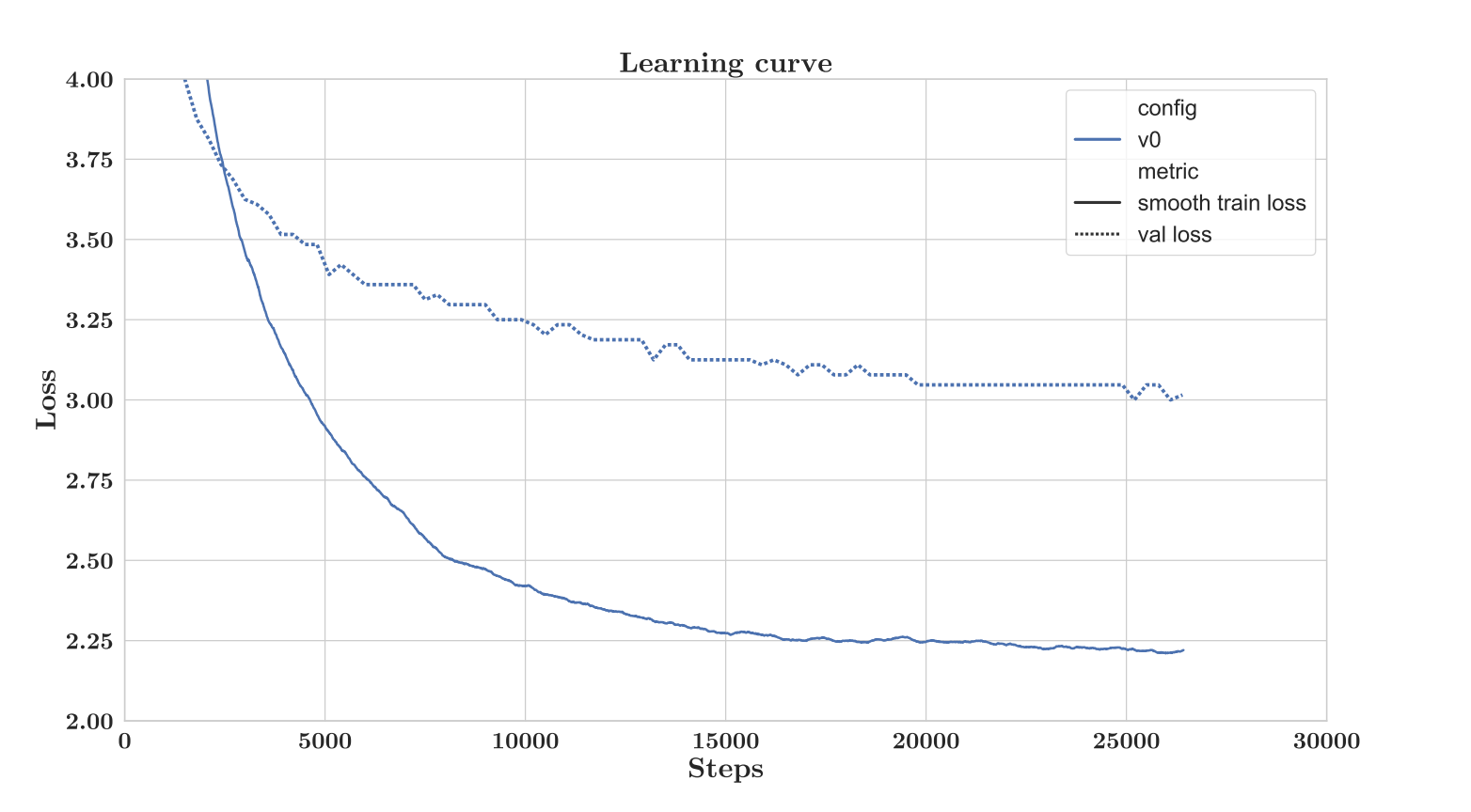
They suspected that the large gap between training and validation and the loss plateau could be due to the chronological sorting of the data. The data in the validation is from a future time period which may have a different distribution than what the model sees during training. They decided to shuffle the data.
v1.x
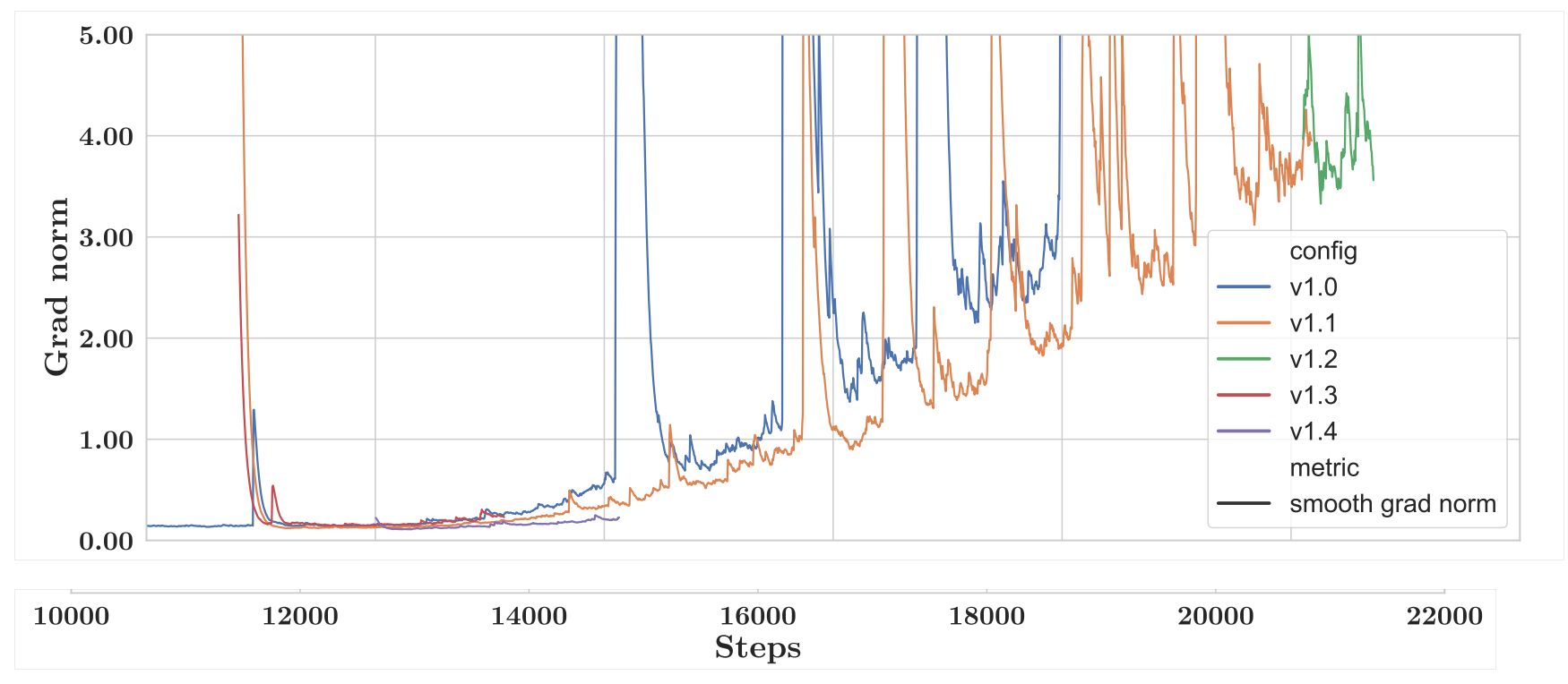
A series of iterations and improvements are made after v0. In order to have a better understanding of where the instability comes from, similar to Meta's OPT model, the Bloomberg team plots the gradient norms across training steps to monitor for training instability.
The figure below shows this for different iterations of the v1 model. Spikes are an indicator of training instability and poor performance.
v1.0: In blue is the model trained after shuffling the data. As seen there is a peak around step 14k.
v1.1: Again borrowing from OPT's learnings, they rewound training to before the spike happened (around 100 steps before), shuffled the next batches of data and lowered the learning rate. As seen, the orange curve, the spike just got delayed.
A Deeper Dive into Parameter Values
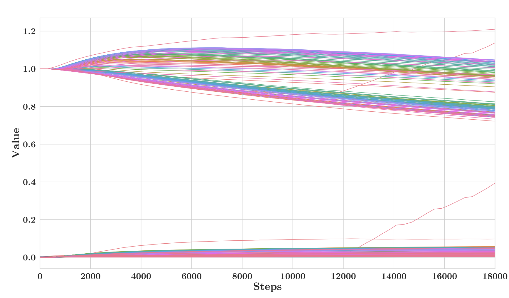
The team suspected that these spikes in the gradient norm to have repercussions in the parameter values. So they plotted the L2 norms for each component, averaged by the square root of the number of elements. As seen in the figure below, most components follow an expected trend. However, the Input LayerNorm at layer 1, elbows and a makes a sudden turn upwards.
They took a deeper look into the values of the multiplier weights $\gamma_1^{in}$. This is the scaling factor when computing the normalisation factor in LayerNorm. All values had the same pattern as seen below:
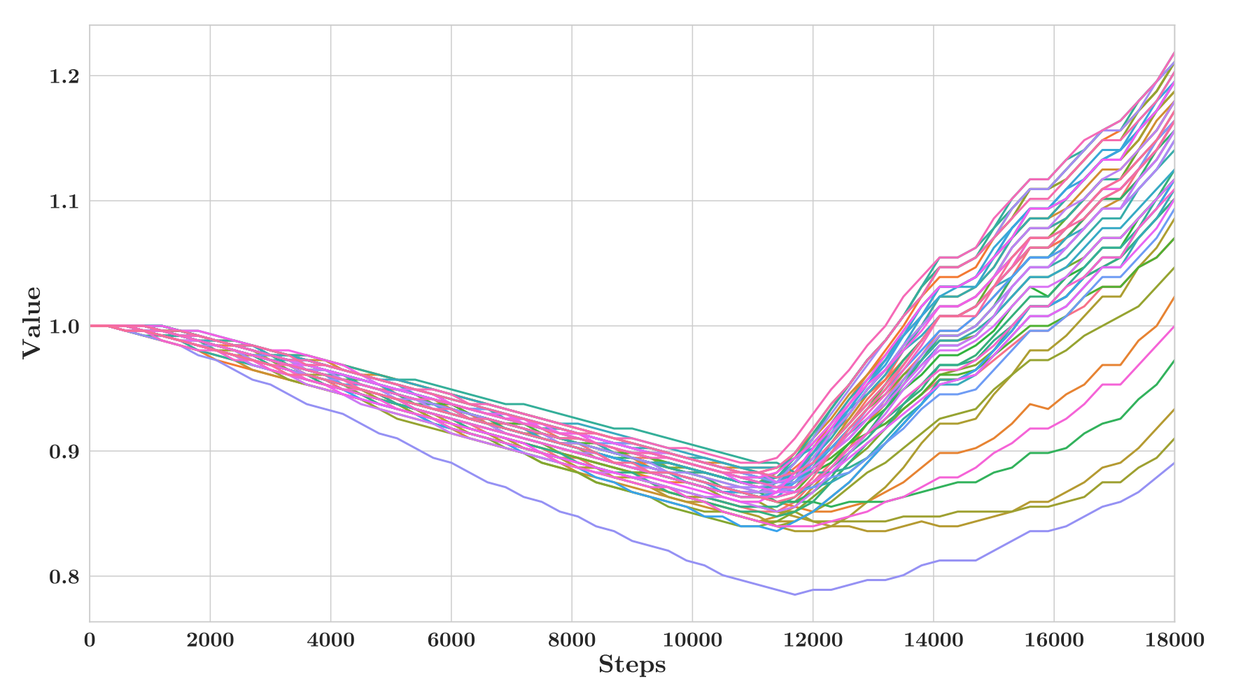
They were not able to figure out what causes this behaviour and after training three more versions of v1, ended up started training from scratch with other hypterparameter changes (The changes are listed in the table below).
However, one thing they noticed from this investigation was that weight decay was beeing applied to the multiplier weights which are initialised at 1. This unnecessarily penalises these values and pulls them to zero. This was removed.
v2
To train the final iteration of the model, the team made a series of hyperparameter choices as listed below:
- Use FP32 precision in LM-head
- Use max learning rate of 6e-5 instead of 1e-4
- Use a gradient clipping value of 0.3 instead of 1.0
- Fully shuffle data
- Use a different seed to ensure different initialization and data order
- Reintroduce LayerNorm at embedding layer (LNem)
- Use a longer learning rate warm-up period of 1800 steps
- Remove incorrect use of weight decay on LayerNorm multipliers
- Use Megatron initialization rescaling
- Apply query key layer scaling Shoeybi et al., 2019
- Apply a batch size warm-up: Use a batch size of 1024 for 7200 iterations, then increase to 2048
They trained this model and monitored norms of weights. For 48 days training went smoothly. However, the training and validation loss flattened from day 41. They made a number of changes, e.g. reducing the learning rate, reducing weight decay and increasing dropout. None of these changes helped and since they had reached the end of their training budget they decided to call it.
Evaluation
The model trained for 48 days was evaluated on a dozen general language tasks, e.g. reading comprehension, knowledge assessments, etc. and compared with LLMs of similar or larger sizes.
Among the models with tens of billions of parameters that we compare to, BloombergGPT performs the best. Furthermore, in some cases, it is competitive or exceeds the performance of much larger models (hundreds of billions of parameters).
In addition to general language tasks the model was evaluated on finance tasks. For example it was used to generate Bloomberg Query Language (BQL) which it did not have in its training data. It was able to generate queries in a few-shot setting.
Takeaways
This paper provides a good example of how to train custom LLMs on proprietary data from scratch. For me the main takeaway was starting small and investigating the issues in the initial iterations before starting the larger scale training. Many of the issues in the larger training setting can be caught in the smaller setting which is much more effective to fix.
I hope you found this article helpful. If you have any questions or feedback, would love to hear from you.