Attention-based nested U-Net (ANU-Net)
In this article, I will be summarising the methods and findings of a paper titled ANU-Net: Attention-based nested U-Net to exploit full resolution features for medical image segmentation, published in May 2020 by Li et. al. This paper uses various techniques to improve the accuracy of medical image segmentation and reduce the prediction time by pruning the model.
Although this paper focuses on medical image segmentation, its techniques can be applied to other applications as the problems these methods solve are general deep learning problems.
Specifically, this paper provides solutions for:
- Vanishing/exploding gradients
- Semantic gap between encoder and decoder feature maps
- Presence of irrelevant features in the feature maps
- Convergence of the model
- Imbalanced training datasets which lead to a biased model
- Slow prediction due to the size of the model and its parameters
This paper has used different techniques to tackle each of these problems which I will discuss in detail in this article. These methods can be used independently, so feel free to skip the parts that are not of your interest (I will refer to the problem number in the headers for easier navigation).
Medical Image Segmentation and its Usage
Imaging segmentation is a subset of computer vision. It is the process of assigning each pixel in the image to a class. A group of pixels that belong to the same class are considered to be part of the same object. The end result of this classification task is a set of contours identifying the different objects in the image.
Medical image segmentation applies this process to medical images such as MRIs and CT scans with the objective to detect abnormalities and lesions in specific parts of the body. This is especially useful in the early detection of cancer. Cancer is the second leading cause of death globally and its early detection and treatment is the main method to increase its survival rate.
ANU-Net's building blocks
Nested, Dense Skip Connections (solution for problems 1&2)
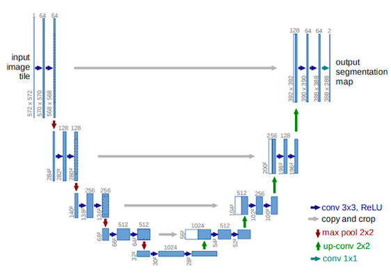
The proposed neural network in this paper, shares its backbone with some previous research. Its main component, similar to many other image segmentation models, is an encoder, decoder structure for downsampling and upsampling the image respectively. This is the U-Net part of the model which was initially proposed by Ronneberger et. al (See Fig.1 from the paper). The name of the network comes from its U shape structure.
Encoders help with detecting what the features are, whereas decoders put these detected features into perspective as to where they are in the input image.
To help with preserving the context of the input and reduce the semantic gap between the encoder and decoder pathways, U-Net concatenates the outputs of each encoder to the decoder of the same depth (see copy and crop arrows in Fig.1).
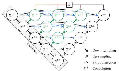
In order to make the encoder and decoder feature maps more semantically similar, Zhou et. al suggested using convolutional layers with dense connections instead of simply concatenating the encoders' feature maps to the decoders (Fig.2 from paper). These layers are called nested skip connections and are densely connected in the sense that the output of each convolutional layer is directly passed the to the next layer (see the dotted blue lines in Fig.2). The idea of densely connected layers was first proposed by Huang et. al and has a number of advantages. It addresses the vanishing gradient issue as the output of all layers including the initial ones get propagated to the higher layers. For the same reason, the model can become more compact. It also, adds more diversity to the feature set as it includes a range of complex features from all the layers.
Attention Gates (solution for problems 2&3)
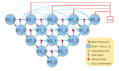
In order to focus on relevant parts of the image and enhance the learning of the target area, Li et. al suggested using attention gates in the skip connections. As seen in Fig.3, the output of each convolutional layer, along with a gate signal get passed to the attention gate to suppress the irrelevant features. More details on how this gate functions is provided below.
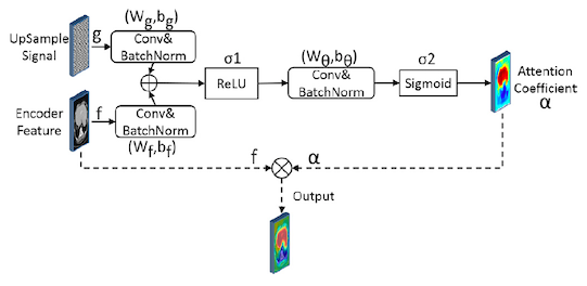
The image below, shows how attention gates are used in this context. This process can be broken down to the following steps:
- Two inputs enter the gate: The gate signal (g), e.g. X2_1 from Fig.3 which is an upsampled feature and helps with selecting more useful information from the second input to the gate: the encoded feature (f), e.g. X1_1
- Convolution and batch normalisation is performed on each input
- The results from step 2 are merged and passed to a relu activation function
- Convolution and batch normalisation
- The result is passed to a sigmoid activation function to compute the attention coefficient $\alpha$
- $\alpha$ is applied to the original feature input to suppress the irrelevant information
Deep Supervision (solution for problem 4)
In order to improve the network's convergence behaviour and have distinct features be selected from all the hidden layers and not just the last layer, Lee et. al suggested Deeply Supervised Nets. The central idea behind this method is to directly supervise the hidden layers as opposed to the indirect supervision provided by backpropagation of the error signal which is computed from the last layer. To achieve this, companion objective functions are placed for each hidden layer.
You can think of this method as truncating the neural network into $m+1$ smaller networks ($m$ being the number of hidden layers) where each hidden layer acts as the final output layer. Therefore, for each hidden layer a loss is computed from the companion objective function. The goal is to minimise the entire network's output classification error while reducing the prediction error of each individual layer.
Backpropagation of error is performed as usual, with the main difference being the the error backpropagates from both the final layer and the local companion output.
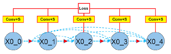
In ANU-Net, the authors have used this idea by adding a $1\times1$ convolutional layer and sigmoid activation function to every output in the first layer and passing the result directly to the final loss function as seen in Fig.5.
Loss function (solution for problem 5)
Up to this point I have discussed the techniques ANU-Net uses to extract full resolution semantic information. In order to learn from this information, a hybrid loss function is used. This function combines two loss functions, Dice loss and Focal loss.
Dice coefficient which is used to compute Dice loss (Dice loss = 1-Dice coefficient) measures the overlap between two samples and is computed as follows:
Where $\bar Y$ is the ground truth and $Y$ is the prediction.
Focal loss focuses on solving the imbalanced dataset problem, a common issue with medical images as with many other fields. It is formulated as below:
- It assigns a weight, $\alpha_t$, to the loss value of the data points. This weight is inversely proportional to the size of the data in each class. So the prediction loss of a point that is from a class that makes up 80% of the entire training set will shrink in value when training because it gets multiplied by $\alpha_t = 1/0.8$. In other words, it forces the loss function to pay more attention to the value of data points from the smaller class.
- It penalises samples that are easily classified ($(1-p)^\gamma$ term, $\gamma$ is set to 2). With this term, Focal loss prevents the model to learn from data points that are easily classified and focuses on hard examples. The easiness of classifying a sample is determined by its probability of belonging to any class, $p_t$. For instance, when the predicted value of a sample data point is close to 0.99 (indicating it belongs to the positive class), $(1-p_t)^\gamma$ penalises the contribution of this easy sample to the overall loss function.
Using the advantages of both Dice loss and Focal loss, ANU-Net proposes the loss function below:
Where $\frac{\alpha \times \bar Y \times logY_i}{|Y_i - 0.5|^\gamma}$ is inspired by Focal loss, the term $\alpha$ has the same objective of down-weighing the dominant class and $\frac{1}{|Y_i - 0.5|^\gamma}$ is the penalising term that assigns higher values to more uncertain inputs. For example, when a data point is assigned a probability of 0.5 (which can belong to either the positive or negative class) this term will be very large forcing the loss function to learn from this hard example.
Note that $s$ is a smoothing factor in the Dice coefficient.
Model Pruning (solution for problem 6)
One huge benefit of using deep supervision is that during inference the model can be pruned. This is because at training, each hidden layer is treated as an output layer with a loss function that backpropagates the error. Since at inference time only forward propagation is done, we can prune the model making it significantly smaller and faster to compute the results. The figure below shows the ANU-Net at four levels of pruning. The grey area are the inactivated section.
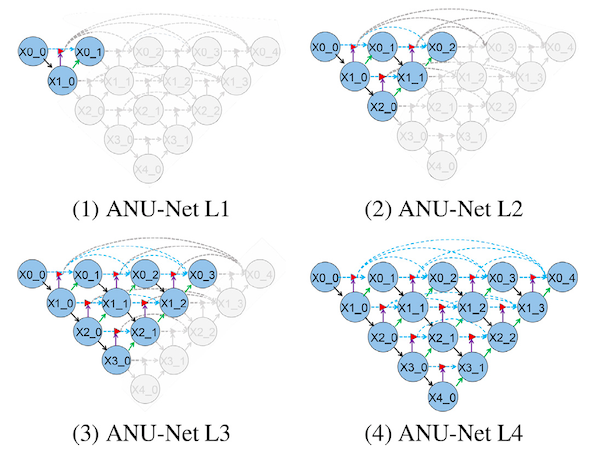
Depending on the performance on the test set, a shallow pruned model with less parameters can be used instead of the full model to increase speed.
Results
Four medical image datasets and four performance metrics namely, Dice, intersection over union (IoU), Precision and Recall were used in this research paper. The results are compared to five popular models (U-Net, R2U-Net, UNet++, Attention U-Net and Attention R2U-Net).
In all four datasets, ANU-Net outperforms the other methods. For instance, in one of the datasets that included CT images of the liver, compared to the Attention U-Net (an older model), ANU-Net's IoU ratio increased by 7.99%, the Dice coefficient increased by 3.7%, the precision increased 5% and recall rate increased 4% (see paper for detailed results).
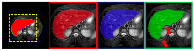
Fig.7 shows the ground truth image for liver segmentation (in red) and compares the results of ANU-Net (in blue) with R2U-Net (in green). The arrows in the rightmost image indicates the areas that R2U-Net missed.
Results from different pruned networks
Note that there is a significant difference in the number of parameters of the pruned and full model. ANU-Net L1 is 98.8% smaller than ANU-Net L4 and when tested on the liver dataset, L1 was 17.13% faster on average at prediction. This speed improvement obviously comes at the cost of accuracy, with a 13.35% and 27.18% decrease in IoU and Dice coefficient respectively. Another pruned model, ANU-Net L3, showed more promising results with a 7.7% increase in speed, 75.5% reduction in parameters and only 0.62% decrease in IoU and 2.56% decrease in Dice coefficient.
Conclusion
In this article, I discussed ANU-Net and its properties. This work, combined very interesting ideas to extract full resolution semantic information with the use of densely connected skip connections, attention gates and deep supervision. It also, used a hybrid loss function that penalises different data points based on the class they belong to and whether they are easily classified or not. In addition, the authors showed the possibility of pruning the model at inference time to speed up prediction. Although this network focuses on medical image segmentation, its components can be applied to any deep learning problem.
I hope you enjoyed learning about these different concepts. If you like reading about machine learning, natural language processing and brain-computer interface, follow me on twitter for more content!