Energy-based Out-of-distribution Detection

In this article, I'm going to summarise a paper with the above title that was published in October 2020. This paper focuses on a common problem in machine learning, overconfident classifiers. What do I mean by that?
Neural networks are a common solution to classification problems. Take the classic digits classification on MNIST handwritten images as an example. With an image dataset of digits from zero to nine, we can train a model that would detect what number is in a given image. But what if the input is a picture of a dog?
Ideally, the model should be able to detect that the features extracted from the dog image is nothing like that of the images it has seen before which were only pictures of numbers. In other words, the model should detect that the dog picture is out of distribution (OOD) and say this doesn't look like anything I have seen before, so I'm not sure if it belongs to any of the 10 classes I was trained on. But that's not what happens. The model which is most likely using a softmax score, outputs the most likely digit class the dog image belongs to, i.e. the model is overconfident.
So what's the solution? Energy scores!
I get into the details of what this score is below but essentially the idea is that softmax scores do not align with the probability density of the inputs and sometimes can produce overly high confidence scores for out-of-distribution samples (hence the model is overconfident), whereas energy scores are linearly proportional to the input distribution. Therefore, they are more reliable in detecting in- and out-of-distribution data points.
This paper shows that energy scores can easily be used at inference time on a pre-trained neural network without any need for changing the model parameters or it can be implemented as a cost function during training.

What is an energy function?

The idea of energy scores comes from thermodynamics and statistical mechanics, specifically from Boltzmann (Gibbs) distribution which measures the probability of a system being in a particular state given the state's energy level and the system's temperature:

Where $T$ is the temperature and $E(x): R^D \rightarrow R$ is the energy function that maps an input of dimension $D$ to a single scalar called the energy value and based on the Helmholtz free energy definition, it can be expressed as:

From Softmax to Energy Function

Now let's consider the softmax function that maps logits of dimension D to K real-valued numbers representing the likelihood of the input belonging to any of the K classes:

  Where $f_{y}(x)$ is the $y^{th}$ index of $f(\mathbf x)$, i.e. the logit representing the $y^{th}$ class. Compare Eq.1 with Eq.3 and we get:

Plug that into the definition of $E(\mathbf{x})$ in Eq.2:

Eq.5 means that without any change in the trained neural network's configuration, we can compute the energy values of the input in terms of the denominator of the softmax function. Now let's see why this helps with the original model overconfidence issue discussed in the introduction.

Using Energy scores instead of softmax scores at inference time

The goal here is to be able to detect when an input is very different from all the inputs used during training. We can look at this as a binary classification problem and use energy functions to compute the density function of our original discriminative model, e.g. handwritten digits classifier:

Take the log of both sides and we get:

The second term in the above equation is simply a constant normalisation factor from the denominator of Eq.6. This proves that the negative energy score of an input $\mathbf x$ is linearly aligned with its density function. In other words, the lower the energy score of some input, the higher the likelihood of it belonging to the input distribution. Fig.1 (from the paper) shows how an energy function as computed by Eq.5 can be applied to a pre-trained model to detect out-of-distribution samples. The energy threshold $\tau$ is set to the value that correctly detects the most number of the in-distribution data (by sliding the negative energy value in the figure below and selecting the number that causes the least overlap between in- and out-of-distribution data).

Linear relation with the probability density is the main reason why energy scores are superior to softmax scores that are not in direct relation with the density function. In fact, the paper shows that the softmax confidence score can be written as the sum of the energy score and the maximum value of $f(\mathbf{x})$. Since $f$ tends to be maximum for seen data and $E(\mathbf {x}; f)$ as shown above is lower for such data, softmax scores are not aligned with the density function.
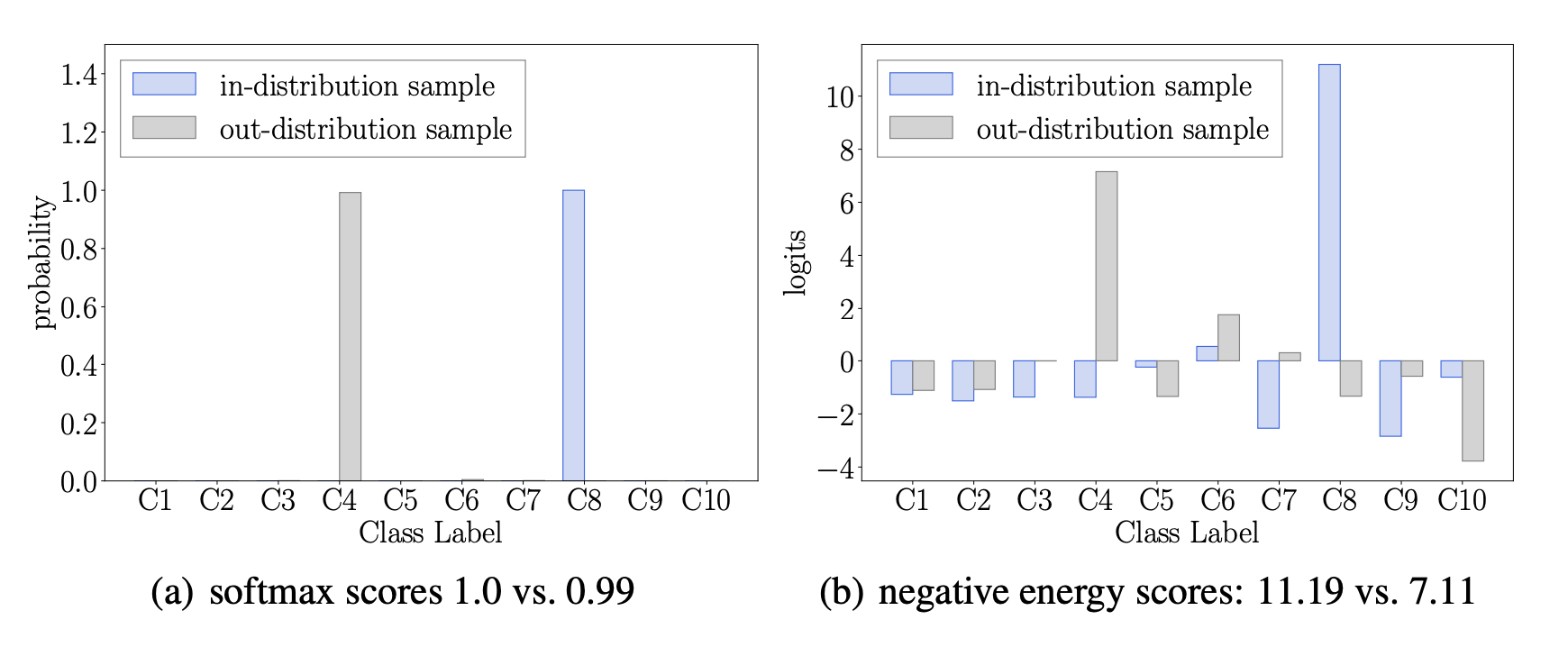
Fig.2 (from the paper) shows the comparison between softmax scores and energy scores for in- and out-distribution data points. The authors split a dataset to training, validation and test and trained a model using the train and validation sets. Then they used the test set as in-distribution samples and used a completely different dataset as out-distribution samples. Notice how the negative energy score for an in-distribution sample is lower and much different than the negative energy score of an out-distribution sample (7.11 vs. 11.19). Whereas, the softmax scores for the same samples are almost identical (1.0 vs 0.99).

Using Energy functions in training

The paper also investigates the benefits of energy-based learning since the gap between in- and out-of-distribution samples in models trained using softmax may not always be enough for accurate differentiation.
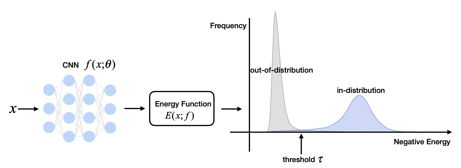
The idea here is that including the energy function in the cost function during training allows for more flexibility to shape the energy surfaces of in- and out-of-distribution data points (blue and grey areas in the right image of Fig.1) and have them far from each other. Specifically, the model is trained using this objective function:

Where $F(\mathbf x)$ is the output of the softmax function, $D^{train}_{in}$ is the in-distribution training data and $L_{energy}$ is a regularisation term based on the energy of in- and out-of-distribution samples used in training. Essentially, this term makes sure that the energy of OOD samples are not below a margin $m_{out}$ and the energy of in-distribution points are not higher than a margin $m_{in}$. In other words, the regularisation loss term makes sure that there is a big enough gap between in- and out-of-distribution samples by penalising samples that have energy levels between $m_{in}$ and $m_{out}$.

Experiments and Results

The authors have used three image datasets, namely SVHN, CIFAR-10 and CIFAR-100 as in-distribution data and six datasets (Textures, SVHN, Places365, LSUN-Crop, LSUN-Resize, iSUN) as out-of-distribution data and measure different metrics. One metric that was considered was the false positive rate (FPR) of OOD examples when the in-distribution true positive rate (TPR) is 95%.
Using energy scores at inference on two pre-trained models, the FPR95 decreased by 18.03% and 8.96% compared to the FPR from the softmax confidence score.
Using energy functions to shape the energy surfaces during training gives less error rates compared to other methods (4.98% vs 5.32%)
The parameter $T$ showed to affect the gap between in- and out-of-distribution samples with an increase bringing the distributions closer to each other. The authors suggest using a value of 1 to make the energy score parameter-free.

Conclusion

This study has shown the shortcomings of current methods used in practice for classifying problems and suggests energy-based learning to improve the models' OOD detection by reducing the false positive rates.
I hope you enjoyed learning about energy scores and their importance. If you like reading about machine learning, natural language processing and brain-computer interface, follow me on twitter for more content!