Do wide and deep networks learn the same things? Uncovering how neural network representations vary with width and depth

When designing deep neural networks we have to decide on its depth/width. These so-called hyper-parameters need to be tuned based on the dataset, available resources, etc. Different studies have compared the performance of wider networks with deeper networks (Eldan et. al & Zagoruyko et. al) but there has been less focus on how these hyper-parameters affect the model beyond its performance. In other words, we do not know enough about how tweaking the network depth/width changes the hidden layer representations and what neural networks actually learn from additional layers/channels.
In this article I am going to summarise the findings of a paper published by Google Research in October 2020. This study investigates the impact that increasing the model width and depth has on both internal representations and outputs. Particularly, it aims at answering the following questions:
- How does depth and width affect the internal representations?
- Is there any relation between the hidden representations of deeper/wider models and the size of the training dataset?
- What happens to the neural network representations as they propagate through the model structure?
- Can wide/deep networks be pruned without affecting accuracy?
- Are learned representations similar across models of different architectures and different random initialisations?
- Do wide and deep networks learn different things?
Each section will answer one of these questions, in order.
Experimental Setup
As mentioned in the intro, this paper focuses on the tensors that passed through the hidden layers and how they change with additional layers, etc. In order to be able to compare the internal representations of different model architectures with one another, some similarity metric is needed. In this work, the authors use linear centered kernel alignment (CKA). This metric was first introduced by Google Brain as a means to understand the behaviour of neural networks better. Please refer to this paper for details on how CKA is computed, but generally speaking you can think of it as any other similarity metric such as cosine similarity that computes the closeness of two tensors. I will get into more detail of CKA when answering question 3.
A family of ResNet models and three commonly used image datasets, CIFAR-10, CIFAR-100 and ImageNet have been used for experiments.
Effect of Increasing Depth/Width on Internal Representations (Question 1)
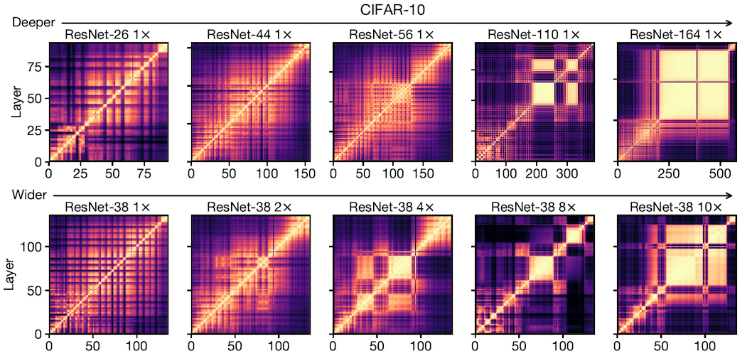
In order to study the impact of width/depth on hidden layers, a group of ResNets is trained on CIFAR-10. For each network, the representation similarity between all pairs of hidden layers is computed. This pairwise similarity measure, gives us a heatmap with the x and y axis representing the layers of the model. The top row of Fig.1 shows such results from 5 ResNets with varying depth (the rightmost being the deepest) and the bottom row shows the outputs of such computations with a different set of ResNets that vary in their width (the rightmost being the widest). As we see, the heatmaps initially resemble a checkerboard structure. This is mainly because ResNets have residual blocks and therefore, representations after residual connections are similar to other post-residual representations. However, things start to get quite interesting as the model gets deeper or wider. We see that with deeper and wider networks, a block structure (yellow squares) starts to appear in the heatmaps suggesting that a considerable number of hidden layers share similarities with each other.
It's worth noting that residual connections are not related to the emergence of block structures as they also appear in networks without them. In addition, the authors compute heatmaps for a deep and a wide model with various random initialisations and see that the block structure is present for each trained model; however, its size and position varies.
Relationship between the block structure and the model size (Question 2)
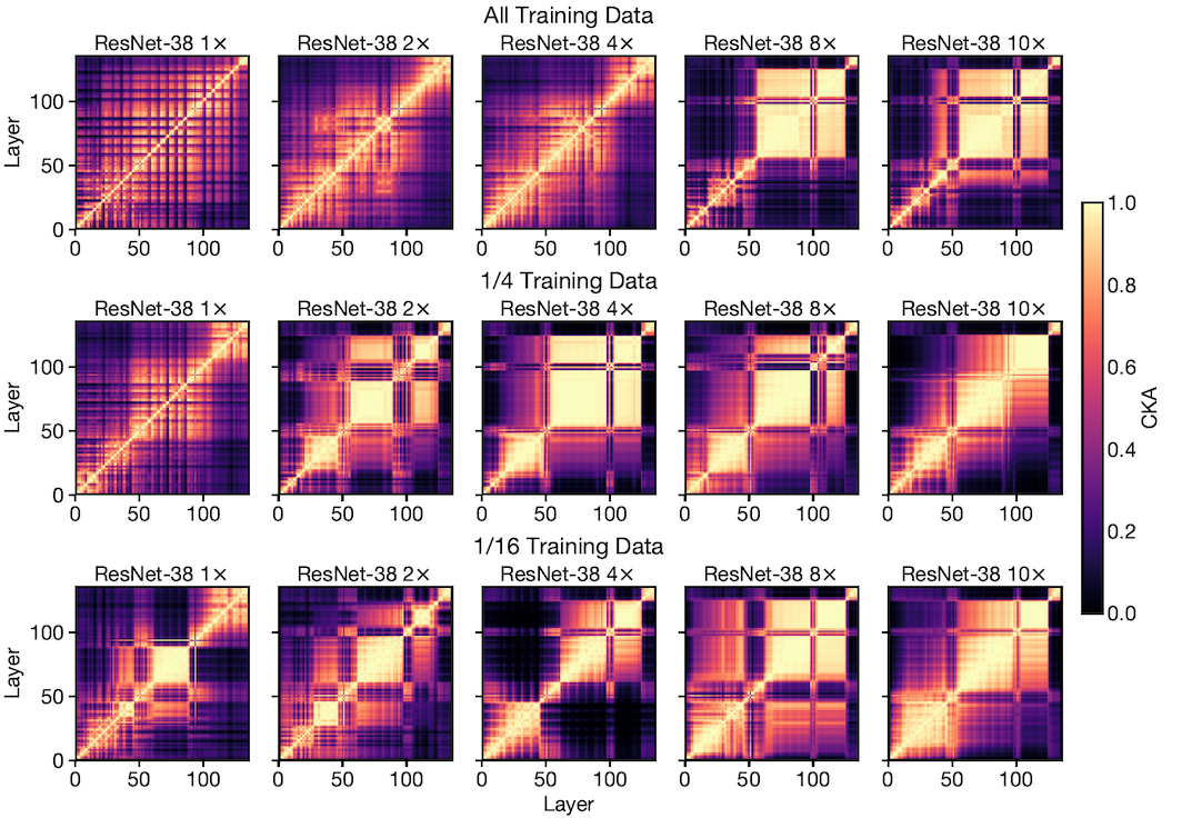
After discovering the emergence of block structures in deeper/wider networks, the authors want to see whether this phenomenon is related to the absolute size of the model or to its relative size to the amount of training data.
In order to answer this question, a model with a fixed architecture is trained on a dataset of varying size. After training, CKA similarity is computed between hidden layer representations as we see in Fig.2. Each column in Fig.2 is a particular ResNet architecture that has been trained on all, 1/4 and 1/16 of the dataset respectively. Each successive column is wider than the previous one. Considering each row, we see that similar to Fig.1, block structure appears as the network gets wider. However, for each model with a fixed width (the columns), block structures emerge when less training data is available.
Experiments on networks with varying depth give similar results (See paper's appendix).
This experiment shows that models that are relatively overparameterised (compared to the amount of training data) contain block structures in their internal representations.
The block structure and the first principal component (Question 3)
So far we have seen block structures emerge in networks as they get wider or deeper and become overparameterised relative to their training data, but we do not know what they actually mean and what information they contain?
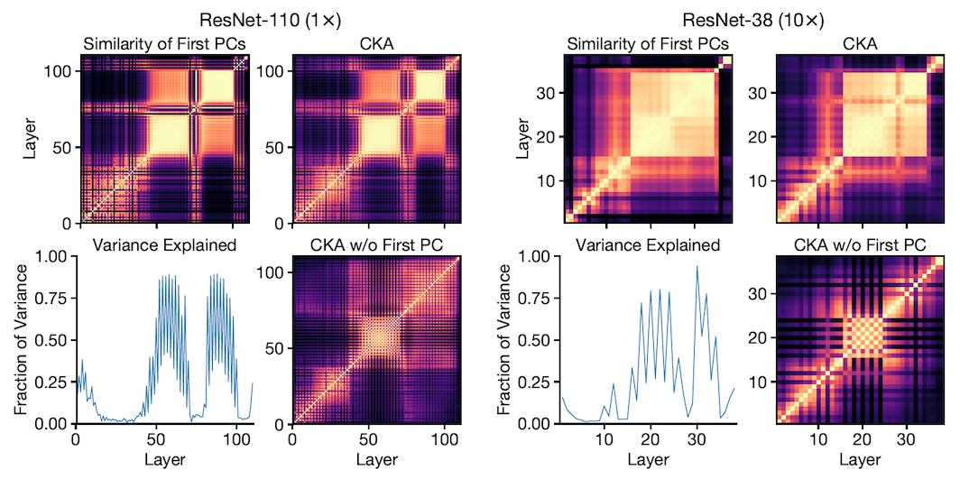
Google Brain's paper on CKA shows that for centered matrices, the CKA can be written in terms of the normalised principal components (PC) of the inputs (See eq.1).
The objective of principal components is to explain as much variance in the data as possible through a set of orthogonal vectors, i.e. principal components. Given eq.1, assuming that the first principal explains all the variance in the data and therefore we only consider this principal component in the summation, the numerator and denominator will cancel each other out and CKA will be equal to $<{\mathbf {u_X}^1, \mathbf {u_Y}^1>}^2$, which is the squared alignment between the first PCs of the inputs.
This led to the idea that the layers with high CKA similarity (block structures) will likely have a first PC that explains a large fraction of the variance of the hidden layer representations. In other words, the block structure reflects the behaviour of the first PC of the internal representations. To verify this, the authors compute the fraction of variance explained by the first PC of each layer in both wide and deep ResNets and see whether a block structure appeared for the same group of layers that covered most of the variance. Fig.3 shows the results. The left set of plots are from a deep network and plots on the right show outputs from a wide network. As we see in both sets, the same group of layers that make up the block structure in the top right heatmaps, cover a high fraction of variance shown in the bottom left graphs.
To further investigate the relation between block structures and first PCs, the cosine similarity between the first PC of all the layers are computed as we see in the top left plots. This shows that the block structures appear in the same size and location as in the heatmaps from CKA (top right).
In addition, authors remove the first PC and compute the CKA heatmap. As illustrated in the bottom right plots, without the first PC the block structures are also removed.
These experiments suggest that the first principal component is what is preserved and propagated throughout its constituent layers leading to block structures.
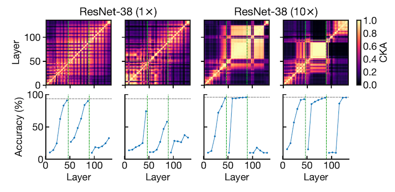
Linear probes and pruning the model (Question 4)
Given that block structures preserve and propagate the first PC, you might be wondering if a) the presence of a block structure is an indication of redundancy? and if so b) whether models that contain block structures in their similarity heatmaps can be pruned?
To answer these two questions, the authors consider each layer of both a narrow and a wide network and fit a linear classifier to predict the output class. This method was introduced by Alain et al. and is called linear probing. You can think of these probes (classifiers) as thermometers that are used to measure the temperature (performance) of the model in various locations. Fig.4 shows two groups of thin and wide ResNets. The two left panes are two thin networks with different initialisations and as we see the accuracy is monotonically increasing for all layers with or without residual connections (shown in blue and orange respectively). However, for a wide network we see little increase in accuracy of layers within the block structure. Note that without residual connections (orange line) the performance of layers that make the block structure decreases. This suggests that these connections play an important role in preserving target representations in the block structure leading to increased prediction accuracy.
This suggests that there is redundancy in the block structures' constituent layers.
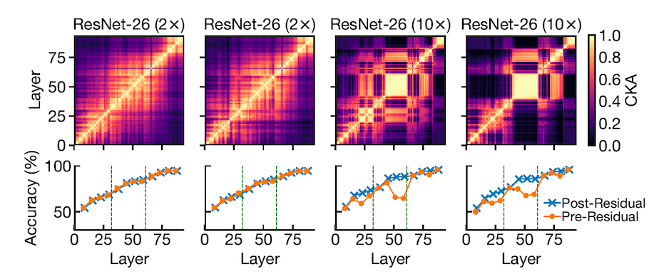
Now let's get to pruning. Note that in ResNets, the network is split into a number of stages. The number of channels and kernel sizes are fixed at each stage and they increase from one stage to the other. The vertical green lines in the bottom row plots of Fig.5 show three stages in the analysed models. In order to investigate the effect of pruning, blocks are deleted one-by-one from the end of each stage while keeping the residual connections since they are important in preserving the important internal representations. Linear probing is performed on intact and pruned models and results show that pruning from inside the block structure (the area between the green vertical lines in the bottom row of Fig.5) has very little impact on the test accuracy. However, pruning has a negative effect on performance for models without block structure. The two left plots in Fig.5 show the comparison in performance between a thin model before and after pruning blocks. We see a noticeable drop in accuracy (blue line in bottom plots) when blocks are removed from any of the three stages.
The two right plots in Fig.5 show the comparison in performance between a wide model with a block structure before and after pruning blocks. We do not see a big difference in accuracy when pruning happens in the middle stage that contains the block structure.
The grey horizontal line shows the performance of the full model.
These results suggest that models that are wide/deep enough to contain a block structure can be compressed without much loss in performance.
Effect of depth/width on representations across models (Question 5)
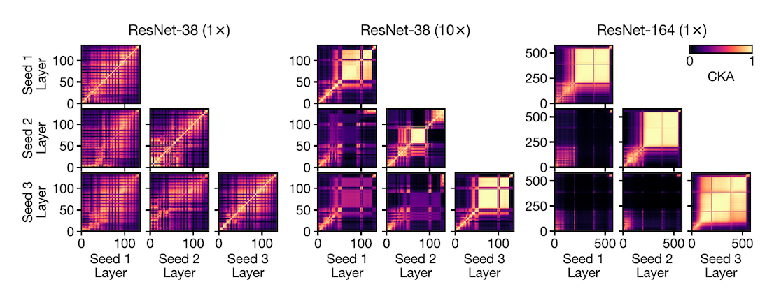
In this section we want to learn a) if models of the same design but different initialisations learn similar representations? and b) whether this changes with increasing the model capacity, i.e. making it deeper/wider? and c) is their similarity between representations of different model designs? and finally d) how is this similarity or dissimilarity affected as models get deeper/wider?
To answer part a, a small model with a fixed architecture was trained three times with three different initialisations. Then, CKA maps between layers of each pair of models was computed (see the leftmost group of plots in Fig.6). As we see in Fig.6, the model does not contain any block structure and representations across initialisations (off-diagonal plots) show the same grid-like similarity structure as within a single model.
The middle (wide model) and right (deep model) group of plots answer part b. Both models have block structures (See plots on the diagonal). Comparing the same model from different seeds (off-diagonal plots) we see that despite some similarity between representations in layers outside the block structure, there is no similarity between the block structures across seeds.
To answer parts c) and d) the same experiments are run on models with different designs. Particularly for part c) two different small model architectures are trained and there similarity is computed. As we see in the left group of plots in Fig.7 for these two models, representations at the same relative depths are similar across models.
However, when comparing a wide and deep model that contain block structures, results show that the representations within the block structure are unique to the model (see group of plots on the right of Fig.7)
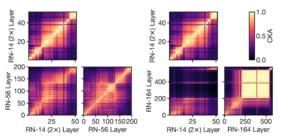
With this analysis, we can conclude that representations from layers outside the block structures bear some resemblance with one another independent of the model architecture being the same or not but there is little to no similarity between representations inside the block structure.
Effect of depth/width on predictions (Question 6)
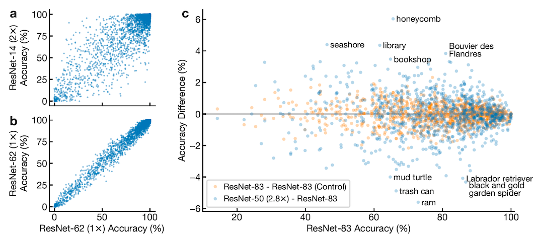
Now we want to investigate the difference between the predictions of different architectures on a per-example basis.
For this purpose, the authors train a population of neural networks on CIFAR-10 and ImageNet. Fig.8a compares the prediction accuracy of individual data points for 100 ResNet-62 (1x) and ResNet-14 (2x) models. As we see the difference in predictions of these models are very different and large enough to not be by chance (Fig.8b). Subplot b suggests that similar model architectures with different initialisations make similar predictions.
Fig.8c shows the accuracy differences on ImageNet classes for ResNets with increasing width (y-axis) and increasing depth (x-axis). This analysis shows that there is a statistically significant difference in class-level error between wide and deep models. On the test sets, wide networks show better performance at identifying scenes compared to objects (74.9% $\pm$ 0.05 vs. 74.6% $\pm$ 0.06, $p = 6 \times 10^5$, Welch’s t-test).
Conclusion
This article goes through the details of a study run by Nguyen et. al which investigated the effect of increasing the capacity of neural networks relative to the training size. They found that with increasing model depth/width, block structures emerge. These structures preserve and propagate the first principal component of the hidden layers. This study also discovered that block structures are unique to each model; however, other internal representations are quite similar across different models or same models with different initialisations. In addition, analysis on different image datasets indicated that wide networks learn different features from deep networks and their class error-level and per-example performance is different.
I hope you enjoyed learning about block structures, when they appear and the difference in performance between wide and deep networks. If you like reading about machine learning, natural language processing and brain-computer interface, follow me on twitter for more content!